Pig Operators – Pig Input, Output Operators, Pig Relational Operators

Input, output operators, relational operators, bincond operators are some of the Pig operators. Let us understand each of these, one by one.

Pig Input Output Operators

Pig LOAD Operator (Input)

The first task for any data flow language is to provide the input. Load operator in the Pig is used for input operation which reads the data from HDFS or local file system.

By default, it looks for the tab delimited file.

For Example X = load ‘/data/hdfs/emp’; will look for “emp” file in the directory “/data/hdfs/”. If the directory path is not specified, Pig will look for home directory on HDFS file system.

If you are loading the data from other storage system say HBase then you need to specify the loader function for that very storage system.

X = load ’emp’ using HBaseStorage();

If we will not specify the loader function then by default it will use the “PigStorage” and the file it assumes as tab delimited file.

If we have a file with the field separated other than tab delimited then we need to exclusively pass it as an argument in the load function. Example as below:

X = load ’emp’ using PigStorage(‘,’);

Pig Latin also allows you to specify the schema of data you are loading by using the “as” clause in the load statement.

X = load ’emp’ as (ename,eno,sal,dno);

If we will load the data without specifying schema then columns will be addressed as $01, $02, etc. While specifying the schema, we can also specify the datatype along with column name details. For Example:

X = load ’emp’ as (ename: chararray, eno: int,sal:float,dno:int);

X = load ”hdfs://localhost:9000/pig_data/emp_data.txt’ USING PigStorage(‘,’) as (ename: chararray, eno: int, sal:float, dno:int);

Pig STORE Operator (Output)

Once the data is processed, you want to write the data somewhere. The “store” operator is used for this purpose. By default, Pig stores the processed data into HDFS in tab-delimited format.

Store processed into ‘/data/hdfs/emp’;

PigStorage will be used as the default store function otherwise we can specify exclusively depending upon the storage.

Store emp into emp using HBaseStorage();

We can also specify the file delimiter while writing the data.

Store emp into emp using PigStorage(‘,’);

Pig DUMP Operator (on command window)

If you wish to see the data on screen or command window (grunt prompt) then we can use the dump operator.

dump emp;

Pig Relational Operators

Pig FOREACH Operator

Loop through each tuple and generate new tuple(s). Let us suppose we have a file emp.txt kept on HDFS directory. Sample data of emp.txt as below:

mak,101,5000.0,500.0,10
ronning,102,6000.0,300.0,20
puru,103,6500.0,700.0,10

Firstly we have to load the data into pig say through relation name as “emp_details”.

grunt> emp_details = LOAD ’emp’ USING PigStorage(‘,’) as (ename: chararray, eno: int,sal:float,bonus:float,dno:int);

Now we need to get the ename, eno and dno for each employee from the relation emp_details and store it into another relation named employee_foreach.

grunt> employee_foreach = FOREACH emp_details GENERATE ename,eno,dno;

Verify the foreach relation “employee_foreach”  using DUMP operator.

grunt> Dump employee_foreach;

Standard arithmetic operation for integers and floating point numbers are supported in foreach relational operator.

grunt> emp_details = LOAD ’emp’ USING PigStorage(‘,’) as (ename: chararray, eno: int,sal:float,bonus:float,dno:int);

grunt> emp_total_sal = foreach emp_details GENERATE sal+bonus;

grunt> emp_total_sal1 = foreach emp_details GENERATE $2+$3;

emp_total_sal and emp_total_sal1 gives you the same output. References through positions are useful when the schema is unknown or undeclared. Positional references starts from 0 and is preceded by $ symbol.

Range of fields can also be accessed by using double dot (..). For Example:

grunt> emp_details = LOAD ’emp’ USING PigStorage(‘,’) as (ename: chararray, eno: int,sal:float,bonus:float,dno:int);

grunt> beginning = FOREACH emp_details GENERATE ..sal;

The output of the above statement will generate the values for the columns ename, eno, sal.

grunt> middle = FOREACH emp_details GENERATE eno..bonus;

The output of the above statement will generate the values for the columns eno, sal, bonus.

grunt> end = FOREACH emp_details GENERATE bonus..;

The output of the above statement will generate the values for the columns bonus, dno.

Bincond or Boolean Test

The binary conditional operator also referred as “bincond” operator. Let us understand it with the help of an example.

5==5 ? 1:2 It begins with the Boolean test followed by the symbol “?”. If the Boolean condition is true then it will return the first value after “?” otherwise it will return the value which is after the “:”. Here, the Boolean condition is true hence the output will be “1”.

5==6 ? 1:2 Output, in this case, will be “2”.

We have to use projection operator for complex data types. If you reference a key that does not exist in the map, the result is a null. For Example:

student_details = LOAD ‘student’ as (sname:chararray, sclass:chararray, rollnum:int, stud:map[]);

avg = FOREACH student_details GENERATE stud#’student_avg’);

For maps this is # (the hash), followed by the name of the key as a string. Here, ‘student_avg’ is the name of the key and ‘stud’ is the name of the column/field.

Pig FILTER Operator

A filter operator allows you to select required tuples based on the predicate clause. Let us consider the same emp file. Our requirement is to filter the department number (dno) =10 data.

grunt> filter_data = FILTER emp BY dno == 10;

If you will dump the “filter_data” relation, then the output on your screen as below:

mak,101,5000.0,500.0,10

puru,103,6500.0,700.0,10

We can use multiple filters combined together using the Boolean operators “and” and “or”. Pig also uses the regular expression to match the values present in the file. For example: If we want all the records whose ename starts with ‘ma’ then we can use the expression as:

grunt> filter_ma= FILTER emp by ename matches ‘ma.*’;

Since, the filter passes only those values which are ‘true’. It evaluates on the basis of ‘true’ or ‘false’.

It is important to note that if say z==null then the result would be null only which is neither true nor false.

Let us suppose we have values as 1, 8 and null. If the filter is x==8 then the return value will be 8. If the filter is x!=8 then the return value will be 1.

We can see that null is not considered in either case. Therefore, to play around with null values we either use ‘is null’ or ‘is not null’ operator.

Pig GROUP Operator

Pig group operator fundamentally works differently from what we use in SQL.

This basically collects records together in one bag with same key values. In SQL, group by clause creates the group of values which is fed into one or more aggregate function while as in Pig Latin, it just groups all the records together and put it into one bag.

Hence, in Pig Latin there is no direct connection with group and aggregate function.

grunt> emp_details = LOAD ’emp’ USING PigStorage(‘,’) as (ename: chararray, eno: int,sal:float,bonus:float,dno:int);

grunt> grpd = GROUP emp_details BY dno;

grunt> cnt = FOREACH grpd GENERATE group,COUNT(emp_details);

Pig ORDER BY Operator

Pig Order By operator is used to display the result of a relation in sorted order based on one or more fields. For Example:

grunt> Order_by_ename = ORDER emp_details BY ename ASC;

Pig DISTINCT Operator

This is used to remove duplicate records from the file. It doesn’t work on the individual field rather it work on entire records.

grunt> unique_records = distinct emp_details;

Pig LIMIT Operator

Limit allows you to limit the number of records you wanted to display from a file.

grunt> emp_details = LOAD ‘emp’;

grunt> first50 = limit emp_details BY 50;

Pig SAMPLE Operator

Sample operator allows you to get the sample of data from your whole data-set i.e it returns the percentage of rows. It takes the value between 0 and 1. If it is 0.2, then it indicates 20% of the data.

grunt> emp_details = LOAD ‘emp’;

grunt> sample20 = SAMPLE emp_details BY 0.2;

Pig PARALLEL

Pig Parallel command is used for parallel data processing. It is used to set the number of reducers at the operator level.

We can include the PARALLEL clause wherever we have a reducer phase such as DISTINCT, JOIN, GROUP, COGROUP, ORDER BY etc.

For Example: SET DEFAULT_PARALLEL 10; 

Meaning is that all MapReduce jobs that get launched will have 10 parallel reducers running at a time.

It is important to note that parallel only sets the reducer parallelism while as the mapper parallelism is controlled by the MapReduce engine itself.

Pig FLATTEN Operator

Pig Flatten removes the level of nesting for the tuples as well as a bag. For Example: We have a tuple in the form of (1, (2,3)).

GENERATE expression $0 and flatten($1), will transform the tuple as (1,2,3). 

When we un-nest a bag using flatten operator, then it creates tuples. For Example: we have bag as (1,{(2,3),(4,5)}).

GENERATE $0, flatten($1), then we create a tuple as (1,2,3), (1,4,5)

Pig COGROUP Operator

Pig COGROUP operator works same as GROUP operator. The only difference between both is that GROUP operator works with single relation and COGROUP operator is used when we have more than one relation.

Let us suppose we have below two relations with their data sets:

student_details.txt 

101,Kum May,29,9010101010,Bangalore102,

Abh Nig,24,9020202020,Delhi103,

Sum Nig,24,9030303030,Delhi

employee_details.txt 

101,Nancy,22,London102,

Martin,24,Newyork103,

Romi,23,Tokyo

Now, let us try to group the student_details.txt and employee_details.txt records.

grunt> cogroup_final = COGROUP employee_details by age, student_details by age; 

Output as below:

(22, {(101, Nancy, 22, London)}, {})

(23, {(103, Romy, 23, Tokyo)},{})

(24, {(102, Martin, 24, Newyork)}, {(102, Abh Nig, 24, 9020202020, Delhi), (103, Sum Nig, 24, 9030303030, Delhi)})

(29, {}, {(101, Kum May, 29, 9010101010, Bangalore)})

Pig SPLIT Operator

Pig Split operator is used to split a single relation into more than one relation depending upon the condition you will provide.

Let us suppose we have emp_details as one relation. We have to split the relation based on department number (dno). Sample data of emp_details as below:

mak,101,5000.0,500.0,10

ronning,102,6000.0,300.0,20

puru,103,6500.0,700.0,10

jetha,103,6500.0,700.0,30

grunt> SPLIT emp_details into emp_details1 IF dno=10, emp_details2 if (dno=20 OR dno=30);

grunt> DUMP emp_details1;

mak,101,5000.0,500.0,10

puru,103,6500.0,700.0,10

grunt> DUMP emp_details2;

ronning,102,6000.0,300.0,20

jetha,103,6500.0,700.0,30

Pig Latin Introduction – Examples, Pig Data Types | RCV Academy

In the following post, we will learn about Pig Latin and Pig Data types in detail.

Pig Latin Overview

Pig Latin provides a platform to non-java programmer where each processing step results in a new data set or relation.

For example, X = load ’emp’; Here “X” is the name of relation or new data set which is fed from loading the data set “emp”,”X” which is the name of relation is not a variable however it seems to act like a variable.

Once the assignment is done to a given relation say “X”, it is permanent. We can reuse the relation name in other steps as well but it is not advisable to do so because of better script readability purpose.

For Example:

X = load 'emp';
X = filter X by sal > 10000.0;
X = foreach X generate Ename;

Here at each step, the reassignment is not done for “X”, rather a new data set is getting created at each step.

Pig Latin also has a concept of fields or columns. In the above example “sal” and “Ename” is termed as field or column.

It is also important to know that keywords in Apache Pig Latin are not case sensitive.

For example, LOAD is equivalent to load. But the relations and column names are case sensitive.  For example, X = load ’emp’; is not equivalent to x = load ’emp’;

For multi-line comments in the Apache pig scripts, we use “/* … */” and for single-line comment we use “–“.

Pig Data Types

Pig Scalar Data Types

  • Int (signed 32 bit integer)
  • Long (signed 64 bit integer)
  • Float (32 bit floating point)
  • Double (64 bit floating point)
  • Chararray (Character array(String) in UTF-8
  • Bytearray (Binary object)

Pig Complex Data Types

Map

A map is a collection of key-value pairs.

Key-value pairs are separated by the pound sign #. “Key” must be a chararray datatype and should be a unique value while as “value” can be of any datatype.

For example:

[1#Honda, 2#Toyota, 3#Suzuki], [name#Mak, phone#99845,age#29].

Tuple

A tuple is similar to a row in SQL with the fields resembling SQL columns. In other

In other words, we can say that tuples are an ordered set of fields formed by grouping scalar data types. Two consecutive tuples need not have to contain the same number of fields.

For example:

(mak, 29, 4000.0)

Bag

A bag is formed by the collection of tuples. A bag can have duplicate tuples.

If Pig tries to access a field that does not exist, a null value is substituted.

For Example:

({(a),(b)},{},{(c),(d)},{ (mak, 29, 4000.0)}), (BigData, {Hadoop, Mapreduce, Pig, Hive})

NULLS

A null data element in Apache Pig is just same as the SQL null data element. The null value in Apache Pig means the value is unknown.

Apache Pig Installation – Execution, Configuration and Utility Commands

Apache Pig Installation can be done on the local machine or Hadoop cluster. To install Apache Pig, download package from the Apache Pig’s release page here.

You can also download the pig package from Cloudera or Apache’s Maven repository.

Pig does not need the Hadoop cluster for installation however it runs on the machine from where we launch the Hadoop jobs. It can also be installed on your local desktop or laptop for prototyping purpose. In this case, Apache Pig will run in local mode. If your desktop or laptop can access the Hadoop cluster then you can install the pig package there as well.

Pig package is written using JAVA language hence portable to all the operating systems but the pig script uses bash script, so it requires UNIX /LINUX operating system.

Once you have downloaded the pig, place it in the directory of your choice and untar it using below command:

tar –xvf <pig_downloaded_tar_file>

Apache Pig Execution

You can execute pig script in following three ways:

  1. Interactive mode

pig  -x  local <script.pig>

Runs in the single virtual machine and all files are in the local system

  1. Interactive mode in Hadoop File System

pig  -x

Runs in Hadoop cluster, it is the default mode

  1. Script mode

pig  -x  local
pig  myscript .pig

Script is a text file can be run in local or MapReduce mode

Command Line and their configurations

Pig provides a wide variety of command line option. Below are few of them:

-h or –help

It will list all the available command line options.

-e or –execute

If you want to execute a single command through pig then you can use this option. e.g. pig –e fs –ls will list the home directory.

P or –propertyfile

It is used to specify a property file that a pig script should read.

The below tabular chart shows the return codes used by pig along with their description.

ValueDescription
0Success
1Retriable failure
2Failure
3Partial failure – Used with multi-query
4Illegal arguments passed to Pig
5IOException thrown – thrown usually by a UDF
6PigException thrown – thrown usually by Python UDF.
7ParseException thrown – in case of variable substitution
8an unexpected exception

Grunt

The interactive shell name of Apache Pig is called Grunt. It provides the shell for users to interact with HDFS using PigLatin.

Once you enter the below command on the Unix env where Pig package is installed

pig –x local

The output will be:

grunt>

To exit the grunt shell you can type ‘quit’ or Ctrl-D.

HDFS command in the grunt shell can be accessed using keyword ‘fs’. Dash(-) is the mandatory part when Hadoop fs is used.

grunt>fs -ls

Utility Commands for controlling Pig from grunt shell

Kill jobid

You can find the job’s ID by looking at the Hadoop’s Job Tracker GUI. The above command can be used to kill a Pig job based on the job id.

exec

exec command to run a Pig script in batch mode with no interaction between the script and the Grunt shell.

Example as below:

grunt> exec script.pig

grunt> exec –param p1=myparam1 –param p2=myparam2 script.pig

run

Issuing a run command on the grunt shell has basically the same effect as typing the statements manually.

Run and exec commands are useful for debugging because you can modify a Pig script in an editor and then rerun the script in the Grunt shell without leaving the shell.

NoSQL Column Family Database – Cloud BigTable, NoSQL Database

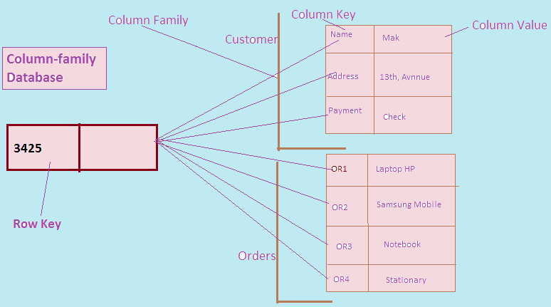
NoSQL column family database is another aggregate oriented database. In NoSQL column family database we have a single key which is also known as row key and within that, we can store multiple column families where each column family is a combination of columns that fit together.

Column family as a whole is effectively your aggregate. We use row key and column family name to address a column family.

It is, however, one of the most complicated aggregate databases but the gain we have in terms of retrieval time of aggregate rows. When we are taking these aggregates into the memory, instead of spreading across a lot of individual records we store the whole thing in one database in one go.

The database is designed in such a way that it clearly knows what the aggregate boundaries are. This is very useful when we run this database on the cluster.

As we know that aggregate binds the data together, hence different aggregates are spread across different nodes in the cluster.

Therefore, if somebody wants to retrieve the data, say about a particular order, then you need to go to one node in the cluster instead of shooting on all other nodes to pick up different rows and aggregate it.

Among the most popular column family NoSQL databases are Apache HBase and Cassandra.

NoSQL Column Family Database
Column Family Database

Aggregate orientation is not always a good thing.

Let us consider the user needs the revenue details by product. He does not care about the revenue by orders.

Effectively he wants to change the aggregate structure from order aggregate line item to produce aggregate line items. Therefore, the product becomes the root of the aggregate.

In a relational database, it is straightforward. We just query few tables and make joins and the result is there on your screen. But when it comes to aggregate orientation database it is a pain.

We have to run different MapReduce jobs to rearrange your data into different aggregate forms and keep doing the incremental update on aggregated data in order to serve your business requirement, but this is very complicated.

Therefore, the aggregate oriented database has an advantage if most of the time you use the same aggregate to push data back and forth into the system. It is a disadvantage if you want to slice and dice data in different ways.

Application of Column family NoSQL Database

Let us understand the key application of column family NoSQL database in real world scenarios.

Big Table (Column Family Database) to store sparse data

We know that NULL values in the relational database typically consume 2 bytes of space.

This is a significant amount of wasted space when there are a number of NULL values in the database.

Let us suppose we have a “Contact Application” that stores username and contact details for every type of the network such as Home-Phone, Cell-Phone, Zynga etc.

If let us say for few of the user only Cell-Phone detail is available then there will be hundreds of bytes wasted per record.

Below is the sample contact table in RDBMS which clearly depicts the waste of space per record.

ContactIDHome-PhoneCell-PhoneEmail1Email2FacebookTwitter
1X2BNULL9867x@abcNULLNULLNULL
2X2B1234NULLNULLNULLNULL#bigtable
3X3Y34569845NULLy@wqaa@fb.com#hadoop
Contact Table in RDBMS

The storage issue can be fixed by using the BigTable which manages sparse data very well instead of RDBMS.

The BigTable will store only the columns that have values for each record instance.

If we indicate only Home-Phone, Cell-Phone and Email1 details that need to be stored for ContactID ‘1X2B’ then it will store only these three column values and rest will be ignored i.e. null will not be considered and hence no wastage of space.

RowKeyColumn Values
1234ph:cell=9867email:1=x@abc
3678social:twitter=#bigtableph:home=1234
5987email:2=y@wqasocial:facebook=a@fb.com
Contact Table in Big Table Storage

Analysing Log File using BigTable

Log analysis is a common use case for any Big Data project. All data generated through log files by your IT infrastructure often are referred to as data exhaust.

The vast information about the logs is stored in big tables. It is then analyzed nearly in real time in order to track the most updated information.

The reason why log files are stored in the BigTable is that they have flexible columns with varying structures.

HostNameIP AddressEvent DTTypeDurationDescription
server110.219.12.34-Feb-15 1:04:21 PMdwn.exe15Desktop Manager
server210.112.3.454-May-15 1:04:21 PMjboss45 
Typical Log File


RowKeyColumn Values
12AE23host:name=server1ip:address
=10.219.12.3
event:DT=4-Feb-15 1:04:21 PMType=
dwn.exe
Dur=15Desc=
Desktop Manager
Log File stored in BigTable

Document Database – Application and Example, NoSQL Database

The main concept behind document database is documents which can be JSON, BSON, XML, and so on. Document database stores documents and retrieves documents.

The data structure defined inside the document databases is hierarchical in nature which can be a scalar value, map or a collection. It is similar to a key-value database but the only difference is that the document database stores the data in form of a document which embeds attribute metadata associated with the stored content.

Document database
Document Database

Every document databases use their own file structure to store data. For example, Apache CouchDB uses JSON to store data, javascript as its query language and HTTP protocol for its API’s.

Document databases are one of the main categories of NoSQL databases. XML databases are a subclass of document databases and are optimized to work with XML documents.

Graph databases are similar to document databases. But graph databases have one more layer, the relationship, which allows graph databases to link documents for rapid traversal.

Among the most popular document databases are MongoDB, Informix, DocumentDB, CouchDB, BaseX.

Application of Document Databases

Let us see an example of the application of document database in the real-world scenario.

Financial derivatives trading service management

Financial Product Markup Language (FpML) is the most common type of document in financial services industry.

They follow an XML schema structure. FpML is mainly used for trading purposes in derivative markets.

Financial institutions need to analyze multiple risk metrics and single view of the customer using the FpML document.

These documents are fed to the document databases and by using the dynamic query language to allow granular access to any data attribute. These databases also allow grouping and reshaping of data through their aggregation framework for their intraday analysis.

These databases also allow grouping and reshaping of data through their aggregation framework for their intraday analysis.