In this section, we will discuss data definition language parts of HIVE Query Language(HQL), which are used for creating, altering and dropping databases, tables, views, functions, and indexes.
We will also look into SHOW and DESCRIBE commands for listing and describing databases and tables stored in HDFS file system.
Hive Database – HIVE Query
A database in Hive is just a namespace or catalog of tables. If we do not specify database, default database is used.
HIVE CREATE database syntax
hive> CREATE DATABASE IF NOT EXISTS financial;
HIVE USE Database syntax
This command is used for using a particular database.
hive> use <database name>

hive> use financial;
HIVE SHOW all existing databases
hive> SHOW DATABASES;

default
financial
For each database, HIVE will create a directory and the tables say “EMP” in that database and say “financial” is stored in sub-directories.
The database directory is created under the directory specified in the parameter “hive.metastore.warehouse.dir”.
Assuming the default value of the parameter is “/usr/hive/warehouse”, when we create the “financial” database, HIVE will create the sub-directory as “/usr/hive/warehouse/financial.db” where “.db” is the extension.
HIVE DESCRIBE database syntax
This will show the directory location of the “financial” database.
hive> DESCRIBE DATABASE financial;

financial
hdfs://usr/hive/warehouse/financial.db
HIVE ALTER Database Syntax
We can associate key-value pairs with a database in the DBPROPERTIES using ALTER DATABASE command.
hive> ALTER DATABSE financial SET DBPROPERTIES (‘edited by’ = ‘kmak’);
HIVE CREATE Table Syntax
CREATE table statement in Hive is similar to what we follow in SQL but hive provides lots of flexibilities in terms of where the data files for the table will be stored, the format used, delimiter used etc.
CREATE TABLE IF NOT EXISTS financial.EMP
(
Ename STRING,
EmpID INT,
Salary FLOAT,
Tax MAP<STRING, FLOAT>,
Subordinates ARRAY<STRING>,
Address STRUCT<city: STRING, state: STRING, zip: INT>
)
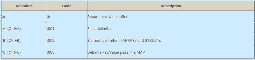
ROW FORMAT DELIMITED
FIELDS TERMINATED BY '\001'
COLLECTION ITEMS TERMINATED BY '\002'
MAP KEYS TERMINATED BY '\003'
LINES TERMINATED BY '\n'
STORED AS TEXTFILE;
In the above example, the default location of the table will be “/user/hive/warehouse/financial.db/EMP”.
If we want to explicitly override the location then we need to use the “LOCATION” keyword in the above create table statement.
HIVE SHOW TABLES Syntax
This command lists the tables in the current working database.
hive> SHOW TABLES;

EMP

Table1

Table2
HIVE DESCRIBE Syntax
The DESCRIBE statement displays metadata about a table, such as the column names and their data types.
hive> DESCRIBE financial.emp.salary

salary    float
HIVE DROP Database Syntax
DROP Database statement deletes all the related tables and then delete the database.
hive>DROP DATABASE IF EXISTS financial;

hive> DROP DATABASE IF EXISTS financial CASCADE;
HIVE DROP Table Syntax
hive> DROP TABLE IF EXISTS emp;
HIVE ALTER Table Syntax
hive> ALTER TABLE emp RENAME TO employee;--Rename Table Name

hive> ALTER TABLE emp CHANGE name firstname String;--Rename Column Name

hive> ALTER TABLE emp CHANGE sal sal Double; -- Rename data types

hive> ALTER TABLE emp ADD COLUMNS (dno INT COMMENT 'Department number'); -- Add column name

hive> ALTER TABLE emp REPLACE COLUMNS (eid INT empid Int,  ename STRING name String);--Deletes all the columns from emp and replace it with two columns
HIVE DESCRIBE EXTENDED Syntax
This command is used for describing details about the table. If we replace EXTENDED with FORMATTED then it provides more verbose output.
The output lines in the description that start with LOCATION also shows the full URL path in the HDFS where hive will keep all the data related to a given table.
hive>DESCRIBE EXTENDED financial.EMP;
Ename STRING,
EmpID INT,
Salary FLOAT,
Tax MAP<STRING, FLOAT>,
Subordinates ARRAY<STRING>,
Address STRUCT<city: STRING, state: STRING, zip: INT>
Detailed Table Information Table( tableName: Emp, dbName:financial, owner:kmak…
Location:hdfs://user/hive/warehouse/financial.db/Emp,
Parameters:{creator=kmak, created at=’2016-02-02 11:01:43’,last_modified_user=kmak,last_modified_time=1443553211,…}HIVE Managed and External Tables
HIVE Managed Tables
By default, HIVE tables are the managed tables. HIVE controls metadata and the lifecycle of the data.
HIVE stores all the data related to a given table in the subdirectory under the directory defined by the parameter “hive.metastore.warehouse.dir” which is “/user/hive/warehouse” by default.
Dropping a managed table deletes the data from the table by deleting the sub-directory that has got created for the respective table. “DESCRIBE EXTENDED” command output will tell whether a table is managed or extended.
The drawback of the managed table is less convenient to use with other tools. For
For Example: We have inserted some data into some table by Pig or some other tool. Now, we wanted to run some HIVE queries on the data inserted by Pig but do not want to give the ownership to HIVE. In such case, we create an external table which has access to the data but not the ownership.
HIVE External Tables
Let us suppose we want to analyze the marketing data getting ingested from different sources.
We ingest south and north zone data using many tools such as Pig, HIVE and so on. Let us assume data file for the SALES table resides in directory /data/marketing.
The following table declaration creates an external table that can read all the data files from /data/marketing distributed directory with data stored as comma-delimited data.
CREATE EXTERNAL TABLE IF NOT EXISTS SALES (
SaleId INT,
ProductId INT,
Quantity INT,
ProdName STRING)

ROW FORMAT DELIMITED FIELDS TERMINATED BY ','
LOCATION '/data/marketing';
The keyword “EXTERNAL” tells HIVE that this table is external and the data is stored in the directory mentioned in “LOCATION” clause.
Since the table is external, HIVE does not assume it owns the data. Therefore, dropping table deletes only the metadata in HIVE Metastore and the actual data remains intact.
Therefore, if the data is shared between tools, then it is always advisable to create an external table to make ownership explicit.
Copy the schema (not the data) of an existing table
CREATE EXTERNAL TABLE IF NOT EXISTS financial.emp1
LIKE financial.emp
LOCATION ‘/data/marketing’;